
Wireshark TCP Stream Graphs: A Practical Guide
 Oliver Ripka
Wireshark's TCP stream graphs turn thousands of packets into a view of how one TCP connection changes over time. They are excellent for finding a stall, a throughput shift, delayed acknowledgment, loss recovery, or a receive-window limit, but a graph is still a visualization of the captured packets, not automatic root-cause proof.
The current TCP Stream Graphs menu provides these main views:
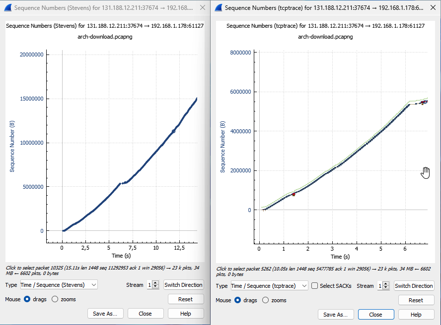
- Time Sequence (Stevens): transmitted sequence space over time
- Time Sequence (tcptrace): data plus ACK, SACK, and advertised receive-window context
- Throughput: throughput calculated over time
- Round Trip Time: ACK-derived RTT samples
- Window Scaling: receive-window behavior, including scaling context
Open the right stream and direction
Select a packet from the connection, then choose Statistics → TCP Stream Graphs and the graph you need. Each graph represents one TCP stream and normally one direction at a time.
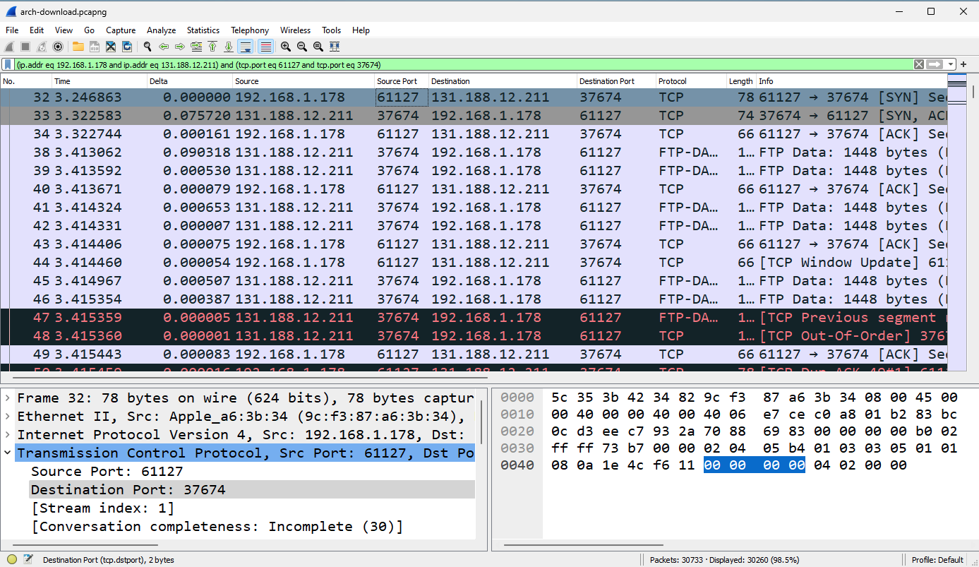
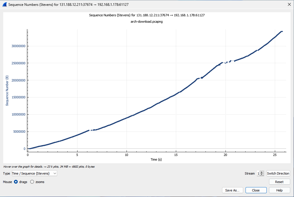
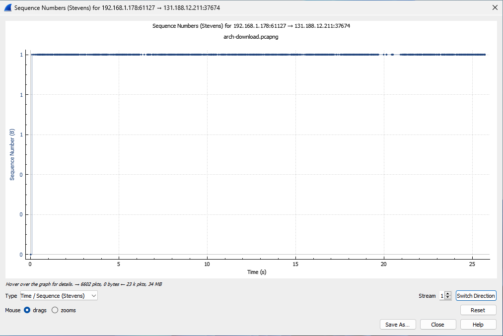
Confirm the source and destination shown in the graph window. Use Switch Direction to inspect the other sender. A download often has a steep data curve in one direction and very little sequence growth in the ACK direction; that is expected.
Time Sequence (Stevens): find when behavior changes
The x-axis is elapsed time. The y-axis is TCP sequence space, measured in bytes. As the sender transmits new bytes, the curve rises.
- A steeper slope means higher throughput.
- A flatter slope means lower throughput.
- A horizontal interval means no new sequence space was sent in that direction.
- A sudden change in slope marks a time worth inspecting in the packet list.
This graph does not by itself distinguish bandwidth limits, congestion control, receive-window pressure, application pacing, or a server pause. It tells you when the transfer changed so you can test those explanations.
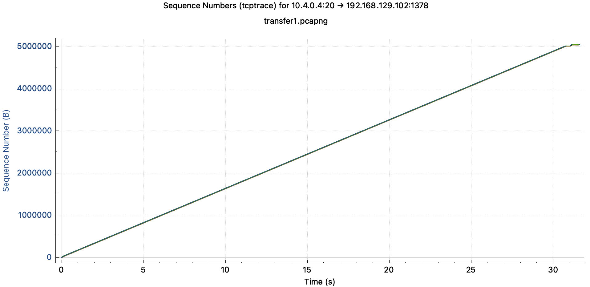
A steady but shallow curve can be a healthy, bandwidth-limited transfer. An irregular curve can still be normal for a paced or bursty application. Always compare the graph with the expected workload and a successful stream.
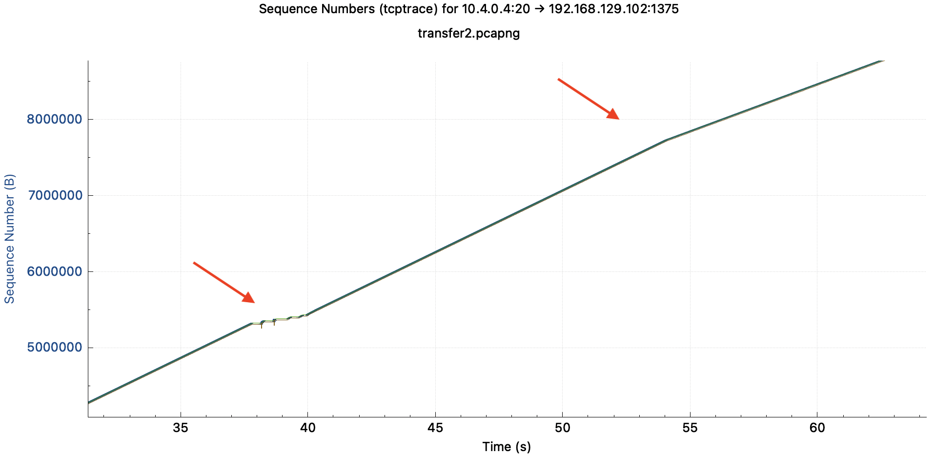
Time Sequence (tcptrace): relate data to receiver feedback
The tcptrace view adds more TCP state around the transmitted data. Depending on Wireshark version and theme, its colors may differ, so use the graph legend and packet linkage rather than memorizing a universal color scheme.
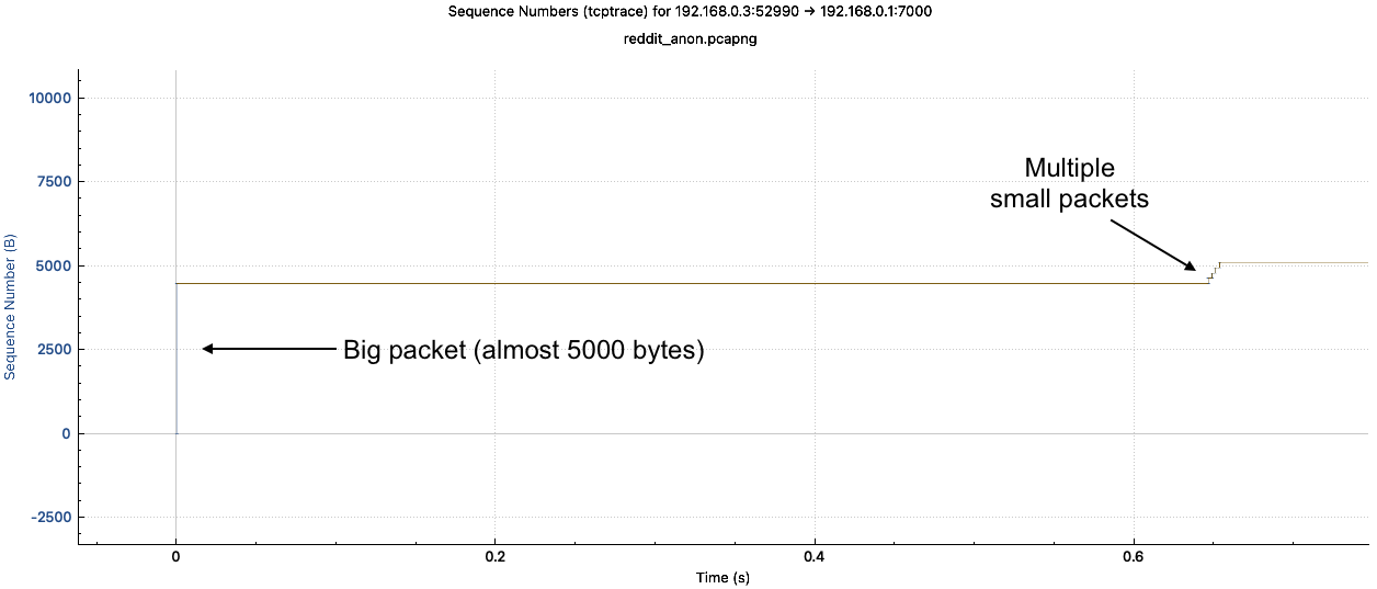
The small vertical data marks span the segment's sequence range. Their height therefore represents the amount of sequence space carried by that segment, not a general “quality” score.
The tcptrace view can also show cumulative ACK progress, SACK ranges, and the receiver's advertised-window boundary. Together they answer three different questions:
- How far has the sender transmitted?
- How far has the receiver cumulatively acknowledged?
- How much additional sequence space is the receiver currently advertising?
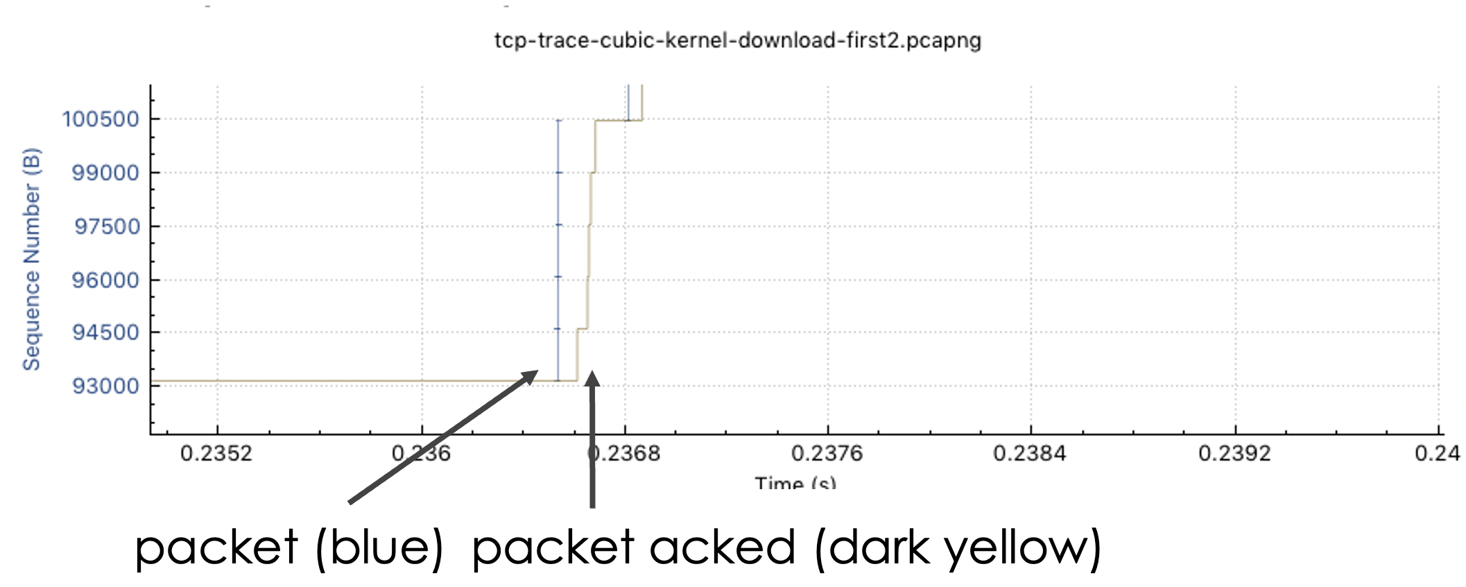
The vertical distance between transmitted data and cumulative ACK progress approximates outstanding sequence space. A persistent gap can reflect RTT, loss recovery, delayed ACK behavior, or capture gaps. It is not automatically packet loss.
Read common patterns carefully
Transfer stall
If new sequence space stops, first identify which constraint is active:
- ACK progress stops while data is outstanding: inspect loss, reordering, RTT, and reverse-path visibility.
- Advertised window reaches the ACK line: the receiver may be window-limited.
- ACKs continue and the window is open, but no new data is sent: investigate application or sender pacing.
- Neither direction is complete in the capture: treat the graph as inconclusive.
Duplicate ACK and fast recovery
Repeated cumulative ACK values can accompany a missing or reordered segment. SACK blocks show which later ranges arrived, helping the sender retransmit the gap without resending everything.
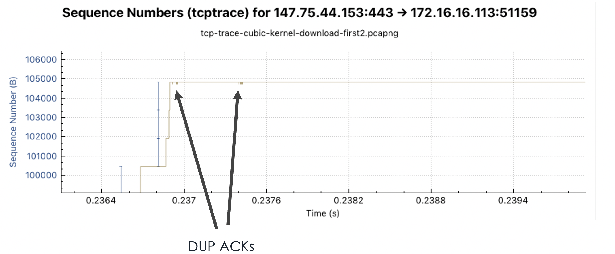
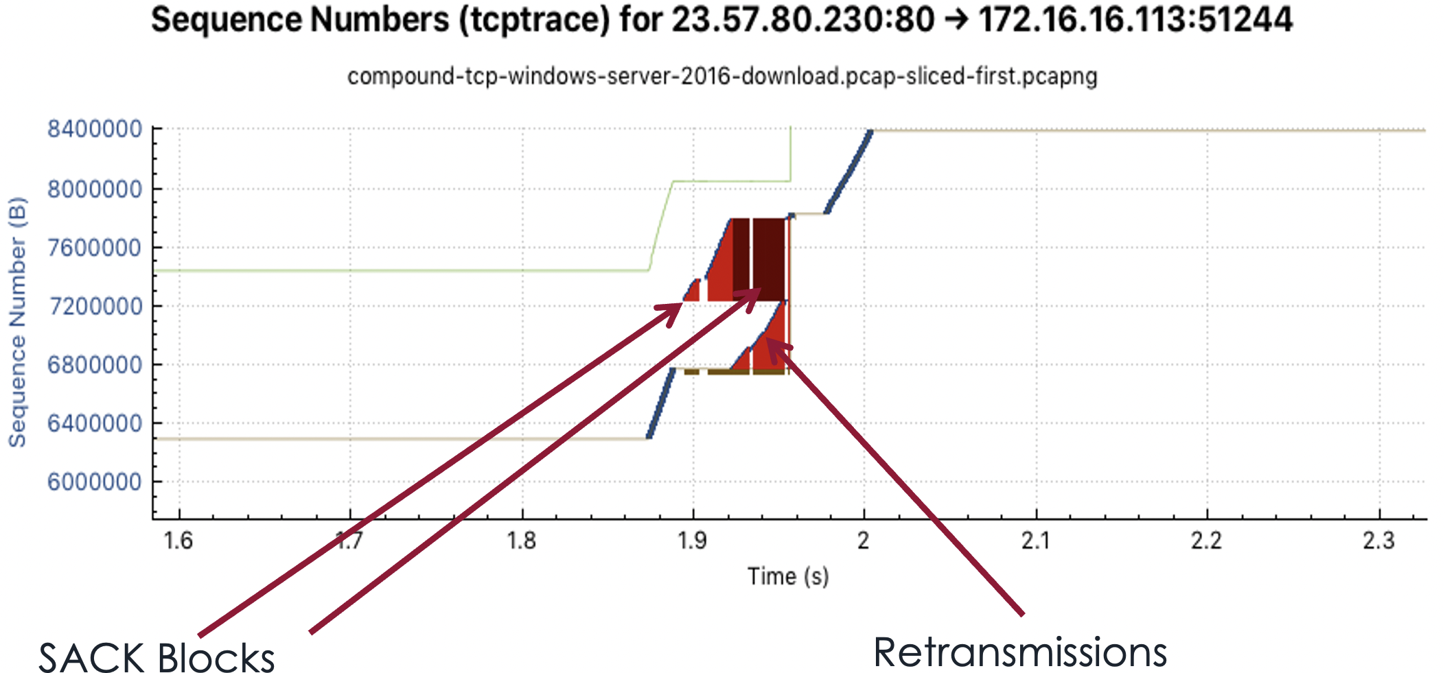
Do not conclude that every duplicate ACK proves network loss. Reordering, duplicated packets, and capture loss can create similar packet-level symptoms. Inspect the missing sequence range and the eventual recovery.
Receive-window pressure
The advertised-window boundary indicates how far beyond the cumulative ACK the sender may transmit. When transmitted sequence space approaches that boundary, the receiver can become the limiting side.
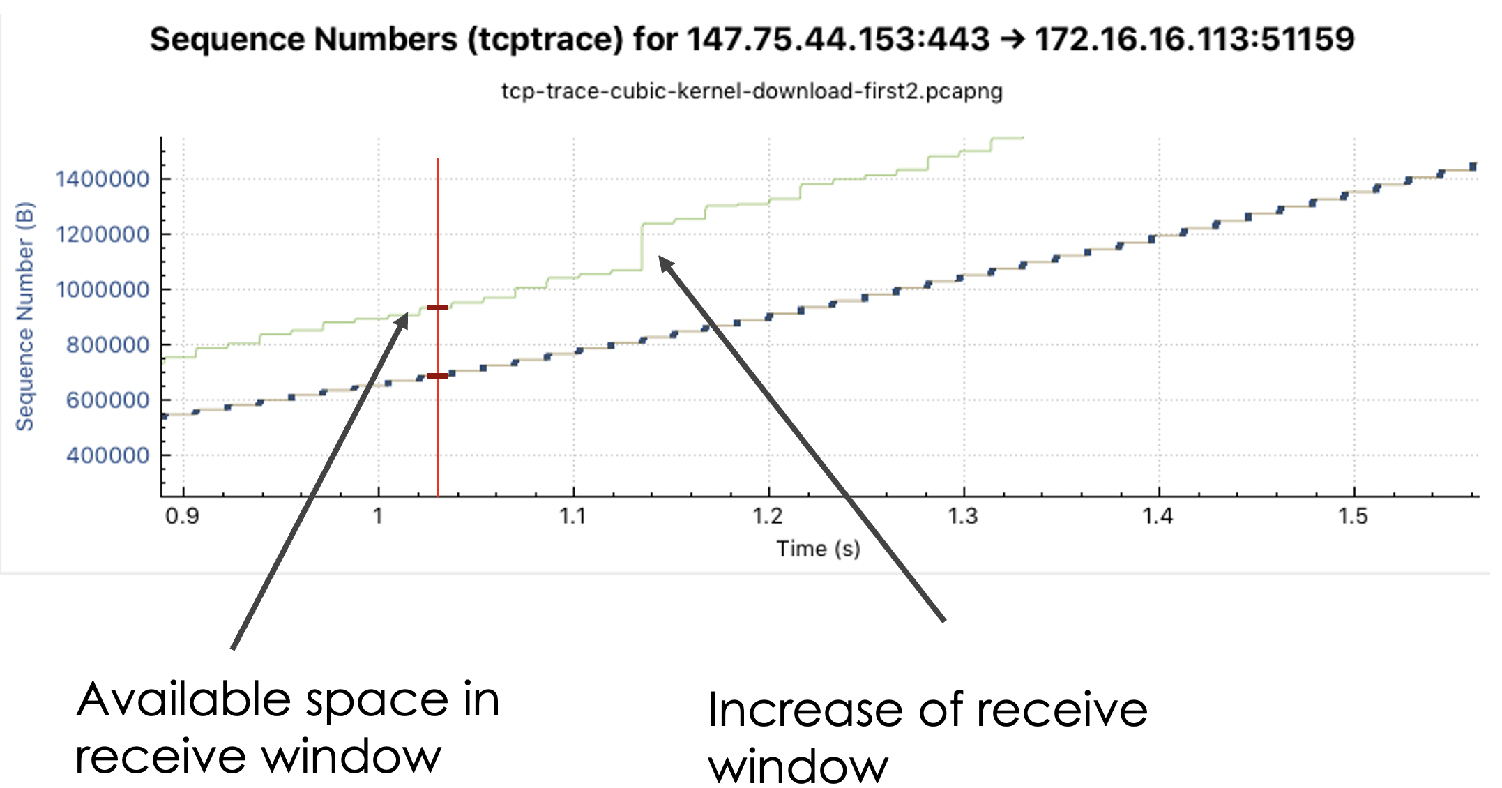
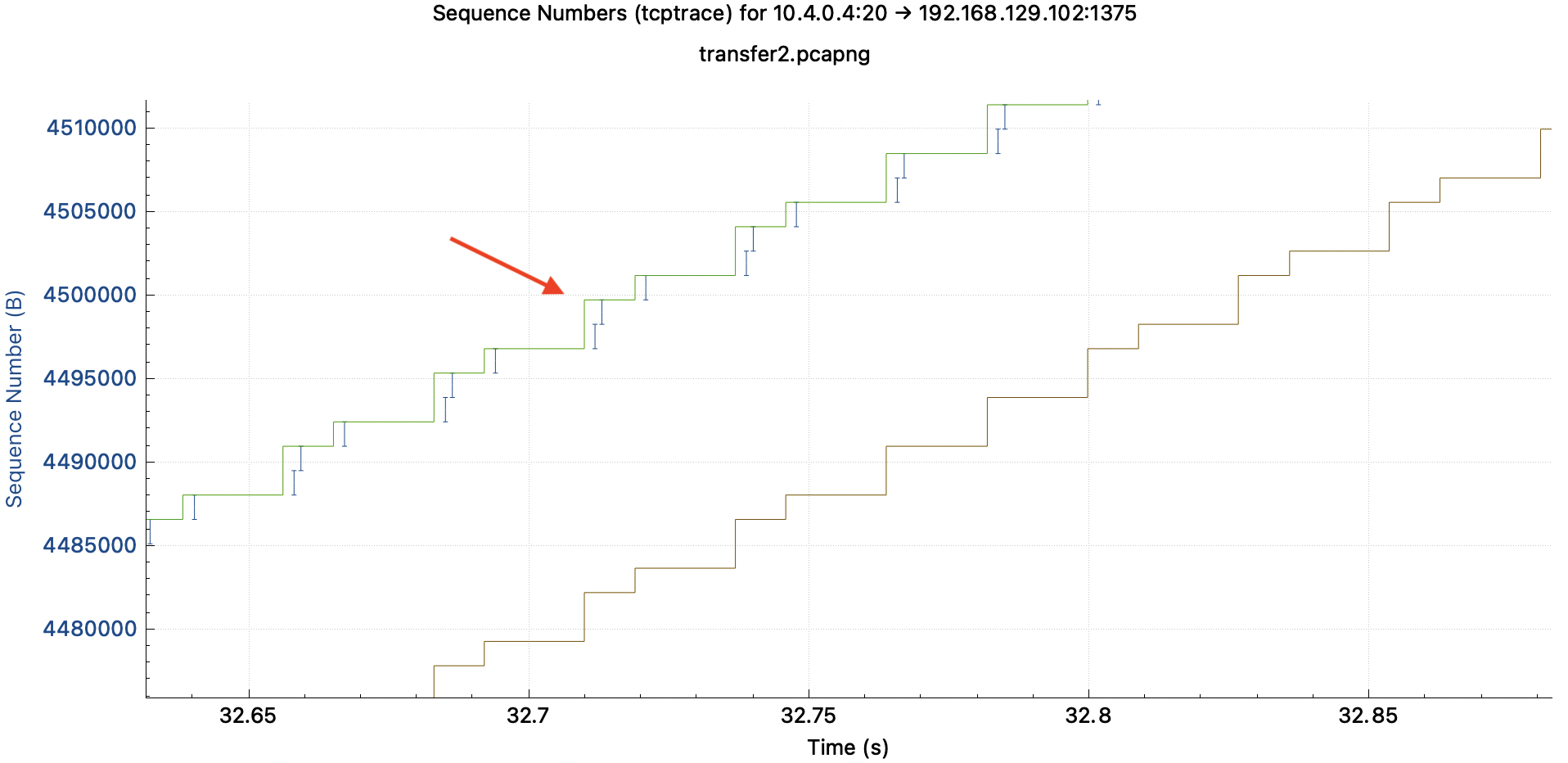
Use these packet fields and analysis labels to verify the graph:
tcp.window_size_value
tcp.window_size_scalefactor
tcp.window_size
tcp.analysis.window_full
tcp.analysis.zero_window
tcp.analysis.window_update
A zero window states that the receiver currently advertises no additional receive space. A “window full” label is Wireshark's interpretation of the visible sequence and window state; confirm direction, scaling, and capture completeness.
Out-of-order arrival versus retransmission
A sequence gap that fills shortly afterward may be reordering or recovery of a lost segment. Timing and receiver feedback distinguish them better than visual shape alone.
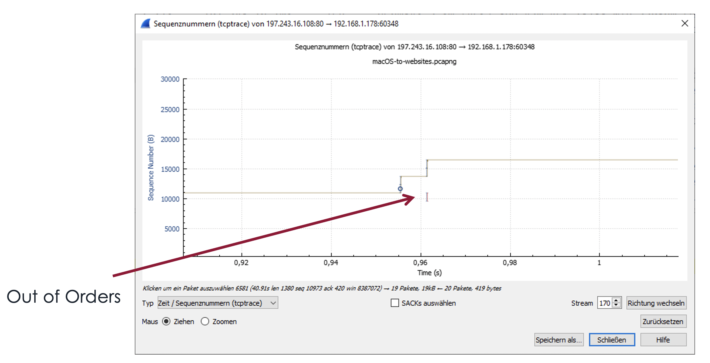
Compare:
tcp.analysis.out_of_order
tcp.analysis.retransmission
tcp.analysis.fast_retransmission
tcp.analysis.spurious_retransmission
tcp.analysis.duplicate_ack
These are calculated analysis fields. Each is a pivot into evidence, not a final verdict.
Use the other graphs to test the hypothesis
Throughput
Use the Throughput graph to quantify when the transfer rate changes. Correlate the interval with sequence/ACK behavior and application messages. Low throughput alone does not identify which layer is limiting the transfer.
Round Trip Time
The RTT graph uses observed data-to-ACK relationships. A rising pattern can support latency, queuing, or recovery pressure, but ACK policy, reordering, and capture position affect samples. Compare the affected stream with a successful connection over the same path.
Window Scaling
Use this view to examine the advertised receive window and scaling behavior. Window scaling is negotiated in the SYN exchange, so a capture that starts midstream may not know the scale factor reliably.
A five-step TCP graph workflow
- Select one affected stream and the data direction. Record endpoints and capture point.
- Use Stevens or Throughput to mark the exact time of the slowdown.
- Use tcptrace to compare transmitted bytes, ACK/SACK progress, and the receive-window boundary.
- Return to the packet list at that time. Validate sequence numbers,
tcp.analysis.ack_rtt, retransmission links, window fields, and application behavior. - Compare a successful baseline. State what the trace proves and what still requires endpoint or infrastructure telemetry.
| Visible pattern | First hypotheses to test | Packet evidence to inspect |
|---|---|---|
| Flat data curve, ACKs and window still advance | Application or sender pause | Application messages, sender timing, zero-length ACKs |
| Flat data curve, ACK progress stops | Loss, reordering, high RTT, missing reverse capture | Sequence gap, SACK, duplicate ACK, tcp.analysis.rto_frame |
| Data approaches advertised-window boundary | Receiver or downstream application pressure | Window scale, zero-window/window-update sequence |
| Repeating recovery bursts | Recurring loss or reordering | Retransmission timing and affected sequence ranges |
| Shallow but steady slope | Bandwidth or deliberate pacing | Throughput baseline, RTT, window headroom |
From graph to evidence-backed report
A useful conclusion should cite the time interval, stream, exact frames or fields, user-visible effect, and a comparison that rejects alternatives. PacketSafari's performance-analysis workflow applies that structure across captures and keeps transport findings reproducible for handoff.
The graph is the map. The packets are the evidence.